Calculation of Fractal Dimension
Chaos and Time-Series Analysis
11/21/00 Lecture #12 in Physics 505
 Comments on Homework
#10 (Time-Delay Reconstruction)
-
Optimum n is about 2 (delay of 2 x 0.05 = 0.1 seconds)
-
This is about equal to autocorrelation time (0.3 seconds) / DE
(3)
-
It's very hard to see fractal structure in return map (D ~ 1.05)
-
Your graphs should look as follows:

 Review (last
week) - Fractals
-
Nonlinear prediction
-
methods usually apply in state space
-
methods can also remove some noise
-
Can be used to produce an arbitrarily long time series
-
Gives an accurate answer to an approximate model
-
Lyapunov exponent of experimental data
-
Getting the LE from experimental data is much more difficult (canned
routines are recommended - See Wolf)
-
Finding a value for LE may not be very useful
-
Noise and chaos both have positive LEs (LE = infinity
for white noise)
-
Quasi-linear dynamics have zero LE, but there are better
ways to detect it (look for discrete power spectrum)
-
Hurst exponent (omitted)
-
Deviation from starting point: DXrms
= NH
-
Hence H is slope of log(DXrms)
versus N (or t)
-
One convention is for white noise to have H = 0
-
And brown noise (1/f 2) to have H = 0.5
-
With this convention, H = a/4 for
1/f a noise
-
Hurst exponent has same information as power law coefficient
 Capacity Dimension
-
The most direct indication of chaos is a strange attractor
-
Strange attractors will generally have a low, non-integer dimension
-
There are many ways to define and calculate the dimension
-
We already encountered the Kaplan-Yorke dimension, but it requires
knowledge of all the Lyapunov exponents
-
Most calculations depend on the fact that amount of "stuff" M scales
as dD
-
Hence D = d log(M) / d log(d) [i.e.,
D
is the slope of log(M) versus log(d)]
-
One example is the capacity dimension (D0)
-
Closely related to the Hausdorf dimension or "cover dimension"
-
Consider data representing a line and a surface embedded
in 2-D
-
The number of squares N of size d required to cover the line
(1-D) is proportional to 1/d
-
The number of squares N of size d required to cover the surface
(2-D) is proportional to 1/d2
-
The number of squares N of size d required to cover a fractal
(dimension D0) is proportional to 1/dD0
-
Hence the fractal dimension is given by D0
= d log(N) / d log(1/d)
-
This is equivalent to D0 = -d log(N)
/ d log(d)
-
Plot log(N) versus log(d) and take the (negative)
slope
to get D0
-
More typically D0 is calculated using a grid of fixed
squares
-
Example (2000 data points from Hénon
map with DE = 2)
-
This derivative should be taken in the limit d --> 0
-
The idea can be generalized to DE > 2 using (hyper)cubes
-
Many data points are required to get a good result
-
The number required increases exponentially with D0
-
If 10 points are needed to define a line (1-D),
then 100 points are needed to define a surface (2-D),
and 1000 points are needed to define a volume (3-D), etc.
 Examples of Fractals
-
There are many other ways to make fractals besides chaotic dynamics
-
They are worthy of study in their own right
-
They provide a new way of viewing the world
-
Fractal slide show (another "lecture within a lecture")
-
Some of these cases will be studied more in the next few weeks
-
Some ways to produce fractals by computer:
-
Chaotic dynamical orbits (strange attractors)
-
Recursive programming
-
Iterated function systems (the chaos game)
-
Infinite mathematical sums (Weierstrass function, etc.)
-
Boundaries of basins of attraction
-
Escape-time plots (Mandelbrot, Julia sets, etc.)
-
Random walks (diffusion)
-
Diffusion limited aggregation
-
Cellular automata (game of life, etc.)
-
Percolation (fluid seeping through porous medium)
-
Self-organized criticality (avalanches in sand piles)
 Similarity Dimension
-
Easy to calculate dimension for exactly self-similar fractals
-
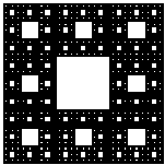
Example #1 (Sierpinski carpet):
-

-
Consists of 9 squares in a 3 x 3 array
-
Eight squares are self-similar squares and one is empty
-
Each time the linear scale is increased 3 x, the "stuff" increases 8 times
Hence, D = log(8) / log(3) = 1.892789261...
-
Note: Any base can be used for log since it involves a ratio
-
Example #2 (Koch curve):
-

-
Consists of 4 line segments: _/\_
-
Each factor of 3 increase in length adds 4 x the "stuff"
Hence, D = log(4) / log(3) = 1.261859507...
-
Example #3 (Triadic Cantor set):
-

-
Consists of three line segments _____ _____ _____
-
Two segments are self similar and one is empty
-
Each factor of 3 increase in length adds 2 x the "stuff"
-
Hence, D = log(2) / log(3) = 0.630929753
 Correlation Dimension
-
Capacity dimension does not give accurate results for experimental
data
-
Similarity dimension is hard to apply to experimental data
-
The best method is the (two-point) correlation dimension (D2)
-
This method opened the floodgates for identifying chaos in experiments
-
Next homework asks you to calculate D2 for the
Hénon map
-
Original (Grassberger and Procaccia) paper included with HW #12
-
Illustration for 1-D and 2-D data embedded
in 2-D
-
Procedure for calculating the correlation dimension:
-
Choose an appropriate embedding dimension DE
-
Choose a small value of r (say 0.001 x size of attractor)
-
Count the pairs of points C(r) with Dr
< r
-
Dr = [(Xi - Xj)2
+ (Xi-1 - Xj-1)2
+ ...]1/2
-
Note: this requires a double sum (i, j) ==> 106
calculations for 1000 data points
-
Actually, this double counts; can sum j from i+1 to N
-
In any case, don't include the point with i = j
-
Increase r by some factor (say 2)
-
Repeat count of pairs with Dr
< r
-
Graph log C(r) versus log r (can use any base)
-
Fit curve to a straight line
-
Slope of that line is D2
-
Think of C(r) as the probability that 2 random points
on the attractor are separated by < r
-
Example: C(r)
versus r for Hénon map with N = 1000 and DE
= 2
-
Result: D2 = 1.223 ± 0.097
-
Compare: DGP = 1.21 ± 0.01 (Original
paper, N = 15,000)
-
Compare: DKY = 1.2583 (from Lyapunov
exponents)
-
Compare: D0 = 1.26 (published result
for capacity dimension)
-
See also my calculations with N
= 3 x 10⁶
-
Generally D2 < DKY<
D0 (but they are often close)
-
Sometimes the convergence is very slow
as r --> 0
-
Tips for speeding up the calculation (in order of
difficulty):
-
Avoid double counting by summing j from i+1 to N
-
Collect all the r values at once by binning the values of Dr
-
Avoid taking square roots by binning Dr2
and using log x2 = 2 log x
-
Avoid calculating log by using exponent of floating point variable
-
Collect data for all embeddings at once
-
Sort the data first so you can quit testing when Dr
exceeds r
-
Can also use other norms, but accuracy suffers
-
Number of data points needed to get valid correlation dimension
-
Need a range of r values over which slope is constant
(scaling region)
-
Limited at large r by the size of the attractor (D2
= 0 for r > attractor size)
-
Limited at small r by statistics (need many points in each
bin)
-
Various criteria, all predict N increases exponentially with
D2
-
Tsonis criterion: N ~ 10 2 + 0.4D
(D to use is probably D2)
| D |
N |
| 1 |
250 |
| 2 |
630 |
| 3 |
1600 |
| 4 |
4000 |
| 5 |
10,000 |
| 6 |
25,000 |
| 7 |
63,000 |
| 8 |
158,000 |
| 9 |
400,000 |
| 10 |
1,000,000 |
J. C. Sprott | Physics 505
Home Page | Previous Lecture | Next
Lecture


