Nonlinear Prediction and Noise Reduction

Comments on Homework #8 (Chirikov Map)

• Everyone had something that resembles Chirikov map
• The map is not normally plotted in polar coordinates despite r and q
• Here's the first few iterations for a square of initial conditions:


• Hard to verify area conservation numerically,

but the stretching is very evident
• Easy to verify area conservation analytically:
• r_n+1 = [r_n - (K/2p) sin(2pq_n)] mod 1 = f(r, q)
• q_n+1 = [q_n + r_n+1] mod 1 = [q_n + r_n - (K/2p) sin(2pq_n)] mod 1 = g(r, q)
• A_n+1/A_n = |det J| = |f_rg_q - f_qg_r| = 1

Review (last week) - Time-Series Properties

• Introductory comments
• Time-series analysis more art than science
• Allows prediction, noise reduction, physical insight
• Easy to get wrong answers
• Hierarchy of Dynamical Behavior
• Regular
• Quasiperiodic
• Chaotic
• Pseudo-random
• Random
• Examples of Experimental Time Series
• Numerical experiments
• Real moving systems
• Abstract dynamical systems
• Non-temporal sequences
• Practical Considerations
• What variable(s) do you measure?
• How much data do you need?
• How accurately must it be measured?
• What is the effect of filtering?
• What if the system is not stationary?
• Case Study
• Two similar signals (one random, one chaotic)
• Both have Gaussian distributions
• Both have flat power spectra (white)
• Hence, this is a bad method for detecting chaos
• It works well for limit cycles (like van der Pol case)

and for N-torus (2 sine waves or 3 sine waves, etc.)
which can be hard to distinguish from chaos
• Instead, look at the return maps (X_n+1 versus X_n)

Autocorrelation Function

• Calculating power spectrum is difficult

(Use canned FFT or MEM  - see Numerical Recipes)
• Autocorrelation function is easier and equivalent
• Autocorrelation function is Fourier transform of power spectrum
• Let g(t) = <x(t)x(t+t)>  (< ... > denotes time average)
• Note:  g(0) = <x(t)²>  is the mean-square value of x
• Normalize:  g(t) = <x(t)x(t-t)> / <x(t)²>
• For discrete data:  g(n) = S X_iX_i+n / S X_i²
• Two problems:
• i + n cannot exceed N (number of data points)
• Spurious correlation if X_av = <X> is not zero
• Use:  g(n) = S (X_i - X_av)(X_i+n - X_av) / S (X_i - X_av)²
• Do the sums above from i = 1 to N - n
• Examples (data records of 2000 points):
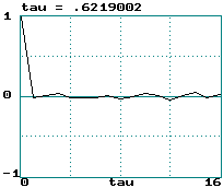
• Gaussian white noise:


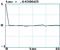
• Logit transform of logistic equation:


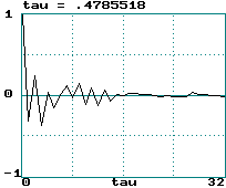
• Hénon map:


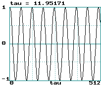
• Sine wave:


• Lorenz attractor (x variable step size 0.05):


• A broad power spectrum gives a narrow correlation function and vice versa

[cf: the Uncertainty Principle (tDf ~ 1)]
• Colored (correlated) noise is indistinguishable from chaos
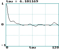
• Correlation time is width of g(t) function (call it tau)
• It's hard to define a unique value of this width
• This curve is really symmetric about tau = 0 (hence width is 2 tau)
• 0.5/tau is sometimes called a "poor-man's Lyapunov exponent"
• Noise:  LE = infinity  ==>  tau = 0
• Logistic map:  LE = log_e(2)  ==>  tau = 0.72
• Hénon map:  LE = 0.419  ==>  tau = 1.19
• Sine wave:  LE = 0  ==>  tau = infinity
• Lorenz attractor:  LE = 0.906/sec = 0.060/step  ==>  tau = 8.38
• This really only works for tau > 1
• Testing this would make a good student project
• The correlation time is a measure of how much "memory" the system has
• g(1) is the linear correlation coefficient (or "Pearson's r")

It measures correlation with the preceding point
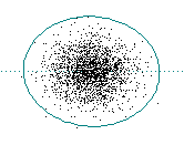
• If g(1) = 0 then there is no correlation

White (f ⁰) noise: 
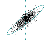
• If g(1) ~ 1 then there is strong correlation

Pink (1/f) noise:
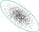
• If g(1) < 0 then there is anti-correlation

Blue (f ²) noise: 
(This was produced by taking the time derivative of white noise)
• From the correlation function g(n), the power spectrumP(f) can be found:

P(f) = 2 S g(n) cos(2pfnDt) Dt  (ref: Tsonis)

Time-Delayed Embeddings

• How do you know what variable to measure in an experiment?
• How many variables do you have to measure?
• The wonderful answer is that (usually) it doesn't matter!
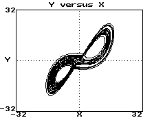
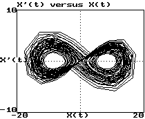
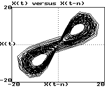
• Example (Lorenz attractor - HW #10):
• Plot of  y versus x:


• Plot of dx/dt versus x:


• Plot of x(t) versus x(t-0.1):


• These look like 3 views of the same object
• They are "diffeomorphisms"
• They have same topological properties (dimension, etc.)
• Whitney's embedding theorem says this result is general
• Taken's has shown that D_E  = 2m + 1
• m is the smallest dimension that contains the attractor (3 for Lorenz)
• D_E is the minimum time-delay embedding dimension  (7 for Lorenz)
• This guarantees a smooth embedding (no intersections)
• This is the price we pay for choosing an arbitrary variable
• Removal of all intersections may be unnecessary
• Recent work has shown that 2m may be sufficient (6 for Lorenz)
• In practice m often seems to suffice
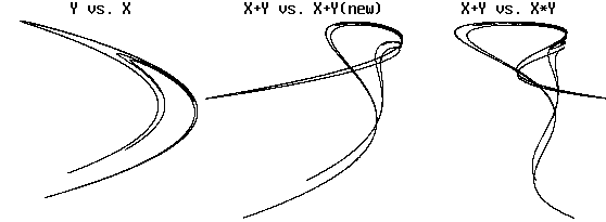
• Example (Hénon viewed in various ways):


There is obvious folding, but topology is preserved
• How do we choose an appropriate D_E (embedding dimension)?
• Increase D_E until topology of attractor (dimension) stops changing
• This may require more data than you have to do properly
• Saturation of attractor dimension is usually not excellent
• Example:  3-torus  (attractor dimension versus D_E , 1000 points)
• Can also use the method of false nearest neighbors:
• Find the nearest neighbor to each point in embedding D_E
• Increase D_E by 1 and see how many former nearest neighbors are no longer nearest
• When the fraction of these false neighbors falls to nearly zero, we have found the correct embedding
• Example: 3-torus
• How do we choose an appropriate Dt for sampling a flow?
• In principle, it should not matter
• In practice there is an optimum
• Rule of thumb:  Dt ~ tau / D_E
• Vary Dt until tau is about D_E  (3 to 7 for Lorenz)
• A better method is to use minimum mutual information (see Abarbanel)

Summary of Important Dimensions

• Configuration space (number of independent dynamical variables)
• Solution manifold (the space in which the solution "lives" - an integer)
• Attractor dimension (fractional if it's a strange attractor)
• Kaplan-Yorke (Lyapunov) dimension
• Hausdorff dimension
• Capacity dimension (see below)
• Information dimension
• Correlation dimension (next week)
• ... (infinitely many more)
• Observable (1-D for a univariate time series: X_i)
• Reconstructed (time-delayed) state space (can be chosen arbitrarily)
• Time-delayed embedding (the minimum time-delayed state space that preserves the topology of the solution)

Nonlinear Prediction

• There are many forecasting (prediction) methods:
• Extrapolation (fitting data to a function)
• Moving average (MA) methods
• Linear autoregression (ARMA)
• State-space averaging (see below)
• Principal component analysis (PCA)

(also called singular value decomposition - SVD)
• Machine learning / AI (neural nets, genetic algorithms, etc.)
• Conventional linear prediction methods apply in the time domain
• Fit the data to a mathematical function (polynomial, sine, etc.)
• The function is usually not linear, but assume that the equations governing the dynamics are (hence no chaos)
• Evaluate the function at some future time
• This works well for smooth and quasi-periodic data
• It (usually) fails badly for chaotic data
• Nonlinear methods usually apply in state space
• Lorenz proposed this method for predicting the weather
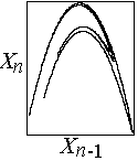
• Example (predicting next term in Hénon map - HW # 11):
• We know X_n+1 = 1 - CX_n² + BX_n-1
• In a 2-D embedding, the next value is unique


• Find M nearest points in X_n-X_n-1 space
• Calculate their average displacement:  DX = <X_n+1 - X_n>
• Use DX to predict next value in time series
• Repeat as necessary to get future time steps
• Sensitive dependence will eventually spoil the method
• Growth of prediction error crudely gives the Lyapunov exponent
• Example (Hénon map average error):


• If LE = 0.604 bits/iterations, error should double every 1.7 iterations
• Saturation occurs after error grows sufficiently
• The method also can remove some noise
• Predict all points not just next point
• Need to choose D_E and M optimally
• Alternate related method is to construct f(X_n, X_n-1, ...)
• This improves noise reduction but is less accurate
• Best method is to make a local function approximation
• Usually linear or quadratic functions are used
• This offers best of both worlds but is hard to implement and slow

Lyapunov Exponent of Experimental Data

• We previously calculated largest LE from known equations
• Getting the LE from experimental data is much more difficult (canned routines are recommended - See Wolf)
• Finding a value for LE may not be very useful
• Noise and chaos both have positive LEs (LE = infinity for white noise)
• Quasiperiodic dynamics have zero LE, but there are better ways to detect it (look for discrete power spectrum)
• The value obtained is usually not very accurate
• Conceptually, it's easy to see what to do:
• Find two nearby points in an embedding D_E
• Follow them a while and calculate <log(rate of separation)>
• Repeat with other nearby points until you get a good average
• There are many practical difficulties:
• How close do the points have to be?
• What if they are spuriously close because of noise?
• What if they are not oriented in the right direction?
• How far can they safely separate?
• What do you do when they get too far apart?
• How many pairs must be followed?
• How do you choose the proper embedding?
• It's especially hard to get exponents other than the largest
• The sum of the positive exponents is called the entropy

Capacity Dimension

• The most direct indication of chaos is a strange attractor
• Strange attractors will generally have a low, non-integer dimension
• There are many ways to define and calculate the dimension
• We already encountered the Kaplan-Yorke dimension, but it requires knowledge of all the Lyapunov exponents
• A more direct method is to calculate the capacity dimension (D₀)
• Capacity dimension is closely related to the Hausdorff dimension
• It is also sometimes called the "cover dimension"
• Consider data representing a line and a surface embedded in 2-D
• The number of squares N of size d required to cover the line (1-D) is proportional to 1/d
• The number of squares N of size d required to cover the surface (2-D) is proportional to 1/d²
• The number of squares N of size d required to cover a fractal (dimension D₀) is proportional to 1/d^D0
• Hence the fractal dimension is given by  D₀ = d log(N) / d log(1/d)
• This is equivalent to  D₀ = -d log(N) / d log(d)
• Plot log(N) versus log(d) and take the slope to get D₀
• Example (2000 data points from Hénon map with D_E = 2)
• This derivative should be taken in the limit d --> 0
• The idea can be generalized to D_E > 2 using (hyper)cubes
• Many data points are required to get a good result
• The number required increases exponentially with D₀