Time-Series Properties

Comments on Homework #7 (Poincaré Sections)

• Some people's Poincaré sections were obviously not correct
• Increasing the damping generally decreases the attractor dimension, eventually leading to a limit cycle.
• Sample results for 0 < b < 0.4

Review (last week) - Hamiltonian Chaos

•  Properties of Hamiltonian (Conservative) Systems
• They have no dissipation (frictionless)
• There are one or more (k) conserved quantities (energy, ...)
• They are described by a Hamiltonian function H

whose  partial derivatives d gives the dynamical equations:
• dx/dt = dH/dv
• dv/dt = -dH/dx
• There are 2N dimensions for N degrees of freedom
• Motion is on a 2N - k dimensional (hyper)surface
• k + 1 Lyapunov exponents are equal to zero
• There are no attractors (or attractor = basin)
• Transients don't die away (no need to wait)
• Equations are time-reversible
• Trajectory returns arbitrarily close to the initial condition
• Phase-space volume is conserved (Liouville's theorem)
• The flow is incompressible (like water)
• The Lyapunov exponents sum to zero
• Chaos can occur only for N > 1 (at least 2 degrees of freedom)
• The dynamics occur in a space of integer dimension
• This space may be a (fat) fractal however (infinitely many holes)
• Example - Chirikov (Standard) Map
• r_n+1 = [r_n - (K/2p) sin(2pq_n)] (mod 1)
• q_n+1 = [q_n + r_n+1] (mod 1)
• K is the nonlinearity parameter
• This system also models ball bouncing on vibrating floor
• Animation of Chirikov map


• Example - Simplest conservative chaotic flow
• dx/dt = y
• dy/dt = z
• dz/dt = x² - y - B
• For B less than about 0.05
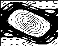
• Poincaré section for B = 0.01

Time-Series Analysis - Introduction

• This is the second major part of the course
• Previously shown:  simple equations often have complex behavior
• This suggests:  complex behavior may have a simple cause
• We move from a theoretical to an experimental viewpoint
• Applications of time-series analysis:
• Prediction, forecasting (economy, weather, gambling)
• Noise reduction, encryption (communications, espionage)
• Insight, understanding, control (butterfly effect)
• Time-series analysis is not new
• Some things are new:
• Better understanding of nonlinear dynamics
• New analysis techniques
• Better and more plentiful computers
• Precautions:
• Time-series analysis is more art than science
• There are few sure-fire methods
• We generally need a battery of tests
• It's easy to fool yourself
• The literature is full of false claims of chaos
• New algorithms are constantly being developed
• "Is is chaos?" might not be the right question

Hierarchy of Dynamical Behavior
(adapted from F. C. Moon)

• Regular predictable behavior (planets, clocks, tides)
• Regular unpredictable behavior (tossing a coin)
• Transient chaos (pinball machine)
• Intermittent chaos (logistic equation)
• Narrow-band (almost periodic) chaos (Rössler attractor)
• Broad-band low-dimensional chaos (Lorenz attractor)
• Broad-band high-dimensional chaos (Mackey-Glass system)
• Correlated (colored) noise (random walk)
• Pseudo-randomness (computer RND function)
• Random (non-deterministic) white noise (radio static)
• Superposition of several of the above (weather, stock market)

Examples of Experimental Time Series

• X_n iterates from an iterated map (i.e., logistic equation)
• x(t) sampled at regular intervals for flow (i.e., Lorenz attractor)
• Population growth (plants, animals)
• Meteorological data (temperature, etc.)
• El Niño (Pacific ocean temperature)
• Seismic waves (earthquakes)
• Tidal levels (good example of N-torus)
• Astrophysical data (sunspots, Cephids, etc.)
• Fluid fluctuations / turbulence (plasmas)
• Financial data (stock market, etc.)
• Physiological data (EEG, EKG, etc.)
• Epidemiological data (diseases)
• Music and speech
• Geological core samples
• Sequence of ASCII codes (written text)
• Sequence of bases in DNA molecule
• Many others ...
• Center of mass of standing human
• Interval between footsteps
• Reaction time intervals
• Necker cube flips


• Eye movements
• Human metronome (tap your foot)
• Attempted human randomness
• Imitate radioactive decay (Geiger counter)
• Write a list of "random numbers"
• Generate a random sequence of bits (0, 1)
• Click mouse at random points on a line

or in a circle or within a square
• The independent variable may not be time, but space, frequency, ...

Practical Considerations

• You may not know the dynamical variables

(or even how many of them there are)
• You may not have experimental access to them
• You may only have a short time record
• The record is usually sampled at discrete times
• The sample rate may not be chosen optimally
• The sample time may be non-uniform

(or some data samples may be missing)
• The data are subject of measuring and rounding errors
• The system may be contaminated by noise
• The signal may be filtered by the detector
• The system may not be stationary (bull market)

Case Study

• Two similar signals (one random, one chaotic)
• Random signal (Gaussian white noise)
• Add N pseudorandom numbers uniform in 0 to 1

(called "uniform deviates")
• Subtract their average (N/2)
• For large N, the result is a Gaussian (normal) distribution with a standard deviation of (N/6)^1/2


• For many purposes N = 6 suffices, but maximum value is only 3.
• Chaotic signal (logit transform of logistic map)
• Generate sequence of iterates from X_n+1 = 4X_n(1 - X_n)
• Transform each iterate by log_e[X/(1 - X)]
• Result approximates a Gaussian distribution


• But it is obviously chaotic (1-dimensional)

(since it came from the logistic map)
• Conventional linear analysis
• Assume signal is sum of sine waves (Fourier modes)
• Example:  looking for "cycles" in stock prices
• Look at power spectrum  P(f)
• Highest f is Nyquist frequency:  f_max = 1/2Dt

(Dt is the time interval between data samples)
• If Dt is too large, aliasing can occur
• Lowest f is approximately:  f_min = 1/NDt

(N is the number of data points)
• If N is too small, data may not be stationary
• White noise has P(f) = constant
• Chaos (i.e., logistic map) can also have P(f) = constant
• Hence, this is a bad method for detecting chaos
• It works well for limit cycles (like van der Pol case)

and for N-torus (2 sine waves or 3 sine waves, etc.)
which can be hard to distinguish from chaos
• Instead, look at the return maps (X_n+1 versus X_n)

Autocorrelation Function

• Calculating power spectrum is difficult

(Use canned FFT or MEM  - see Numerical Recipes)
• Autocorrelation function is easier and equivalent
• Autocorrelation function is Fourier transform of power spectrum
• Let g(t) = <x(t)x(t+t)>  (< ... > denotes time average)
• Note:  g(0) = <x(t)²>  is the mean-square value of x
• Normalize:  g(t) = <x(t)x(t-t)> / <x(t)²>
• For discrete data:  g(n) = S X_iX_i+n / S X_i²
• Two problems:
• i + n cannot exceed N (number of data points)
• Spurious correlation if X_av = <X> is not zero
• Use:  g(n) = S (X_i - X_av)(X_i+n - X_av) / S (X_i - X_av)²
• Do the sums above from i = 1 to N - n
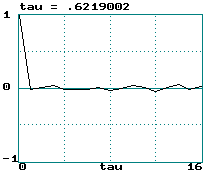
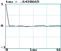
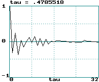
• Examples (data records of 2000 points):
• Gaussian white noise:


• Logit transform of logistic equation:


• Hénon map:


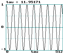
• Sine wave:


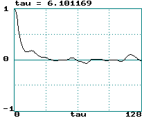
• Lorenz attractor (x variable step size 0.05):


• A broad power spectrum gives a narrow correlation function and vice versa
• Colored (correlated) noise is indistinguishable from chaos
• Correlation time is width of g(t) function (call it tau)
• It's hard to define a unique value of this width
• This curve is really symmetric about tau = 0 (hence width is 2 tau)
• 0.5/tau is sometimes called a "poor-man's Lyapunov exponent"
• Noise:  LE = infinity  ==>  tau = 0
• Logistic map:  LE = log_e(2)  ==>  tau = 0.72
• Hénon map:  LE = 0.418  ==>  tau = 1.20
• Sine wave:  LE = 0  ==>  tau = infinity
• Lorenz attractor:  LE = 1.50/sec = 0.075/step  ==>  tau = 6.67
• This really only works for tau > 1
• Testing this would make a good student project
• The correlation time is a measure of how much "memory" the system has
• From the correlation function g(n), the power spectrumP(f) can be found:

P(f) = 2 S g(n) cos(2pfnDt) Dt  (ref: Tsonis)

Time-Delayed Embeddings

• How do you know what variable to measure in an experiment?
• How many variables do you have to measure?
• The wonderful answer is that (usually) it doesn't matter!
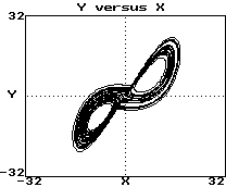
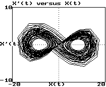
• Example (Lorenz attractor):
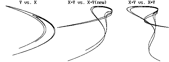
• Plot of  y versus x:


• Plot of dx/dt versus x:


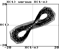
• Plot of x(t) versus x(t-0.1):


• These look like 3 views of the same object
• They are "diffeomorphisms"
• They have same topological properties (dimension, etc.)
• Whitney's embedding theorem says this result is general
• Taken's has shown that D_E  = 2m + 1
• m is the smallest dimension that contains the attractor (3 for Lorenz)
• D_E is the maximum time-delay embedding dimension  (7 for Lorenz)
• This guarantees a smooth embedding (no intersections)
• This is the price we pay for choosing an arbitrary variable
• Removal of all intersections may be unnecessary
• Recent work has shown that 2m may be sufficient (6 for Lorenz)
• In practice m often seems to suffice
• Example (Hénon viewed in various ways):


There is obvious folding, but topology is preserved
• How do we choose an appropriate D_E (embedding dimension)?
• Increase D_E until topology of attractor (dimension) stops changing
• This may require more data than you have to do properly
• Saturation of attractor dimension is usually not excellent
• Example:  3-torus  (attractor dimension versus D_E , 1000 points)
• Can also use the method of false nearest neighbors:
• Find the nearest neighbor to each point in embedding D_E
• Increase D_E by 1 and see how many former nearest neighbors are no longer nearest
• When the fraction of these false neighbors falls to nearly zero, we have found the correct embedding
• How do we choose an appropriate Dt for sampling a flow?
• In principle, it should not matter
• In practice there is an optimum
• Rule of thumb:  Dt ~ tau / D_E
• Vary Dt until tau is about D_E  (3 to 7 for Lorenz)
• A better method is to use minimum mutual information