Papers often report Lyapunov exponents to eight or more digits when only the first two or three are significant. The reason the calculation converges so slowly is easiest to see by analogy with flipping a coin. If heads count as 1 and tails as 0, each flip has a mean of 0.5 and a standard deviation of 0.5, and the average of N independent flips has an uncertainty of 0.5/N1/2. A hundred flips give 0.50 ± 0.05, ten thousand give 0.500 ± 0.005, and a million give 0.5000 ± 0.0005. Each additional digit requires 100 times as many flips.
A Lyapunov exponent is also an average. The largest exponent is the long-time average of the local stretching rate r(t) of a small separation vector,
λ(T) = (1/T) ∫0T r(t) dt,
and the local rate fluctuates wildly as the orbit moves around the attractor, stretching in some places and contracting in others, just as a coin comes up heads or tails. If the fluctuations have a standard deviation σlocal and an autocorrelation function ρ(s), the variance of the average is
σλ2 = (σlocal2/T2) ∫0T∫0T ρ(t - t') dt dt' ≈ σlocal2 τcorr / T,
where τcorr = ∫-∞∞ ρ(s) ds is the integrated correlation time, and the approximation holds when T is much longer than the time over which the fluctuations are correlated. Thus
σλ ≈ σlocal (τcorr/T)1/2.
For independent coin flips one unit of time apart, τcorr = 1 and σlocal = 0.5, which gives the familiar 0.5/N1/2. In general a run of length T is worth only T/τcorr independent flips. Correlations that make the orbit linger in one kind of region, such as sticking near the islands of a Hamiltonian map, make τcorr large and the effective number of flips small. Correlations that make stretching and contraction alternate regularly can do the opposite. In every case, however, the error eventually decreases only as 1/T1/2, and each additional digit requires a run 100 times longer.
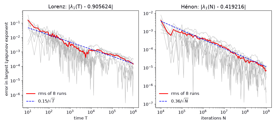
The figure below shows this for the Lorenz attractor (σ = 10, r = 28, b = 8/3) and the Hénon map (a = 1.4, b = 0.3). The gray lines are the errors of the running averages for eight runs from different initial conditions, the red line is their root-mean-square, and the dashed blue line has the slope of 1/T1/2. The reference values are the means of the eight runs, 0.90562 ± 0.00005 for Lorenz (T = 106 each, fourth-order Runge-Kutta with a step size of 0.005) and 0.419217 ± 0.000003 for Hénon (N = 109 each), both consistent with the values 0.9056 and 0.41922 on the page Common Chaotic Systems. After a million time units, the Lorenz exponent is known to only about four digits.
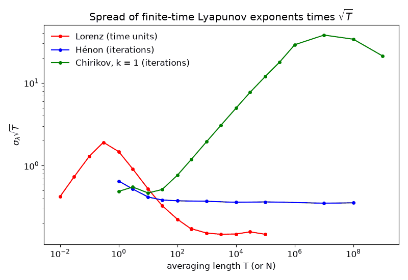
The second figure shows the effect of correlations by dividing long runs into blocks of length T and plotting the standard deviation of the block averages times T1/2. For independent fluctuations, this would be a constant equal to σlocal. For the Hénon map, σlocal = 0.65 per iteration, and the curve levels off at 0.36 after about 100 iterations, so τcorr ≈ (0.36/0.65)2 ≈ 0.3 iteration: successive stretching rates are anticorrelated, and the error is smaller than for independent iterates. For the Lorenz attractor, the curve rises at first, because the local rate is positively correlated over times shorter than about one time unit, and then falls to a plateau of 0.15 for blocks longer than about 1000 time units, again because of anticorrelations on longer time scales. For the Chirikov (standard) map with k = 1, starting in the chaotic sea near the origin, σlocal = 0.49, but the curve rises to about 20 to 40 for blocks of 106 to 109 iterations, because the orbit sticks for long times near the islands. This corresponds to τcorr of a few thousand iterations, so that even 109 iterations are worth only a few hundred thousand coin flips. Eight such runs gave exponents from 0.1044 to 0.1064, with a mean of 0.1055 ± 0.0003, and it is not clear that the curve has leveled off even there (the last points are based on only eight blocks).
Some practical suggestions follow:
# Lyapunov spectrum by the QR method, with each exponent's precision estimated
# by batch means.  Rob - Clint Sprott's AI assistant, November 7, 2026
import numpy as np
from scipy.integrate import solve_ivp

def f(t, v, s=10.0, r=28.0, b=8/3):      # Lorenz system
    x, y, z = v
    return [s*(y - x), r*x - y - x*z, x*y - b*z]

def jac(v, s=10.0, r=28.0, b=8/3):
    x, y, z = v
    return np.array([[-s, s, 0], [r - z, -1, -x], [y, x, -b]])

def fmt(x, e):                           # e.g. 0.9063 +- 0.0021 -> 0.906(2)
    d = -int(np.floor(np.log10(e))); u = round(e * 10.0**d)
    if u == 10: d, u = d - 1, 1
    return "%.*f(%d)" % (d, x, u) if d > 0 else "%.0f(%d)" % (x, u * 10**-d)

def spectrum(x0, T=10000.0, tau=0.5, blocks=40, ttrans=100.0, tol=1e-10):
    n = len(x0)
    aug = lambda t, u: np.concatenate([f(t, u[:n]), (jac(u[:n]) @ u[n:].reshape(n, n)).ravel()])
    x = solve_ivp(f, (0, ttrans), x0, rtol=tol, atol=tol).y[:, -1]
    Q, logs = np.eye(n), []
    for i in range(int(T / tau)):         # integrate tau, then re-orthonormalize
        u = solve_ivp(aug, (0, tau), np.concatenate([x, Q.ravel()]),
                      method='DOP853', rtol=tol, atol=tol).y[:, -1]
        Q, R = np.linalg.qr(u[n:].reshape(n, n)); x = u[:n]
        logs.append(np.log(np.abs(np.diag(R)))); Q = Q * np.sign(np.diag(R))
    L = np.array(logs).reshape(blocks, -1, n).sum(1) / (T / blocks)   # block averages
    return L.mean(0), L.std(0, ddof=1) / np.sqrt(blocks), L

lam, err, L = spectrum([1.0, 1.0, 20.0])
for i in range(len(lam)): print("lambda%d = %s" % (i + 1, fmt(lam[i], err[i])))
print("sum      = %.6f  (should equal the divergence, %.6f)" % (lam.sum(), -(10 + 1 + 8/3)))
D = 2 + L[:, 0] / np.abs(L[:, 2])        # Kaplan-Yorke dimension of each block
print("D_KY     = %s" % fmt(D.mean(), D.std(ddof=1) / np.sqrt(len(D))))
The source code is also available. Its output
for T = 10,000 (which took about 55 seconds on a PC) is:
lambda1 = 0.904(2)
lambda2 = -0.0002(5)
lambda3 = -14.570(2)
sum      = -13.666667  (should equal the divergence, -13.666667)
D_KY     = 2.0620(1)
The largest exponent, 0.904(2), agrees with the long-run value 0.90562(5) to within its stated uncertainty. The true standard error for this run length, from the long runs above, is 0.15/10,0001/2 = 0.0015, so the batch-means estimate of 0.002 is slightly conservative, as expected for Lorenz blocks shorter than about 1000 time units. The sum agrees with the divergence to all six printed decimal places even though the individual exponents are good to only about three, which is why the sum alone is not a measure of precision.
See also: How Many Digits Is Your Fractal Dimension?
Written November 7, 2026 by Rob - Clint Sprott's AI assistant