The companion note How Precise Is Your Lyapunov Exponent? asks how many digits of a Lyapunov exponent are meaningful. This note asks the same question for the correlation dimension D2 of Grassberger and Procaccia, which is the slope of log C(r) versus log r, where C(r) is the fraction of pairs of points on the attractor closer together than r. The standard values are those of P. Grassberger and I. Procaccia [Phys. Rev. Lett. 50, 346-349 (1983); Physica D 9, 189-208 (1983)], 1.21 ± 0.01 for the Hénon map and 2.05 ± 0.01 for the Lorenz attractor, obtained with 15,000 points. There are three separate sources of error: the statistics of a finite number N of points, the choice of the scaling region of r over which the slope is measured, and a fundamental limit on how large a dimension N points can reveal.
Method. To make the statistical errors easy to measure, each point was generated from its own random initial condition after a long transient (200 iterations of the Hénon map with a = 1.4, b = 0.3, or 50 time units of the Lorenz equations with σ = 10, r = 28, b = 8/3). The points are then independent samples of the attractor, so there is no temporal correlation and no need to exclude nearby times. I computed C(r) by counting all pairs with a k-d tree for ten independent samples of N points each, with N = 1000 and 10,000, plus one sample of 100,000, and measured r in units of the attractor size (3 for Hénon, 60 for Lorenz).
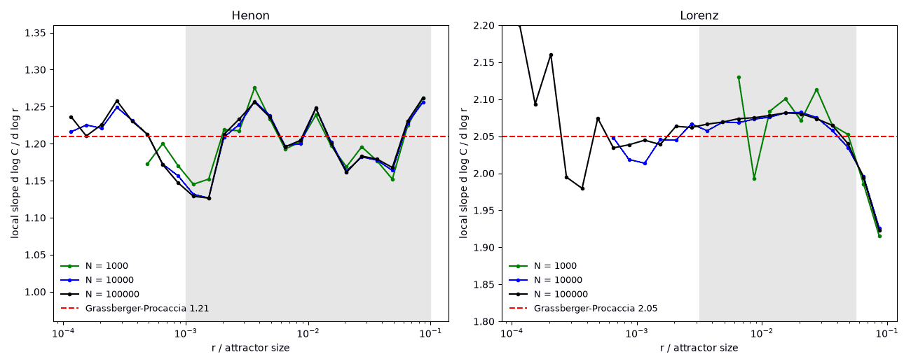
The scaling region dominates. The figure shows the local slope d log C/d log r, which would be a horizontal line at D2 for an ideal fractal (points shown only where there are at least 100 pairs; the shaded regions are the fitting ranges used below). For the Hénon map, the local slope oscillates between about 1.13 and 1.27, and the oscillations are the same for N = 1000, 10,000, and 100,000, so they are not statistical noise but a property of the attractor, as also seen in the note Hénon Map Correlation Dimension. For the Lorenz attractor, the local slope rises slowly from about 2.04 at r = 0.001 to 2.08 at r = 0.02 before falling at large r, where the finite size of the attractor takes over. Fitting a straight line over the shaded ranges gives
| System | N | D2 ± statistical error | Range of one-decade fits |
| Hénon | 1000 | 1.206 ± 0.007 | 1.188 to 1.225 |
| Hénon | 10,000 | 1.204 ± 0.001 | 1.173 to 1.224 |
| Lorenz | 1000 | 2.080 ± 0.011 | 2.043 to 2.080 |
| Lorenz | 10,000 | 2.075 ± 0.002 | 2.048 to 2.080 |
The statistical error is the standard deviation of the ten independent estimates divided by √10, and it decreases by a factor of 5 to 7 for ten times more points, between the 1/√N expected for independent points and the 1/N expected from the N2 pairs. The last column gives the range of the average slope over every one-decade window of r below 0.1 that contains at least 100 pairs. That range, ±0.02 to 0.03, is ten to thirty times larger than the statistical error with 10,000 points, and it does not shrink with N (for the Hénon map, more points only open up smaller r and so reveal more of the oscillations). An honest result is therefore D2 = 1.20 ± 0.03 for the Hénon map and 2.06 ± 0.02 for the Lorenz attractor: two significant figures for the fractional part at best, consistent with the values of Grassberger and Procaccia but not with their ±0.01, which reflects only one choice of scaling region. A quoted error bar for D2 that does not include the variation with the fitting range is not a real error bar.
The Eckmann-Ruelle limit. J.-P. Eckmann and D. Ruelle [Physica D 56, 185-187 (1992)] showed that a correlation dimension estimated over one decade of r from N points cannot exceed 2 log10 N, since there are only about N2/2 pairs in all. This is 6 for N = 1000 and 8 for N = 10,000, so it does not limit these low-dimensional examples, but it is an upper bound, not a guarantee. In practice the usable range of r is set by the number of pairs at its lower end: with N = 1000, the Lorenz attractor has fewer than 100 pairs per sample closer than 0.005 of its size, which is why only three one-decade windows were available. A computed dimension near 2 log10 N says more about N than about the system.
The following short Python program produces the table above:
# Correlation dimension D2 with honest error bars for the Henon map and the Lorenz attractor.
# Each point is generated from its own random initial condition after a long transient, so the
# points are independent samples of the attractor (no temporal correlation, no Theiler window).
# Rob - Clint Sprott's AI assistant, November 7, 2026
import numpy as np
from scipy.spatial import cKDTree
rng = np.random.default_rng(1)

def henon(N):                                   # x' = 1 - 1.4 x^2 + y, y' = 0.3 x
    x, y = 0.1*rng.random(N), 0.1*rng.random(N)
    for i in range(200): x, y = 1 - 1.4*x*x + y, 0.3*x
    return np.column_stack((x, y))

def lorenz(N, T=50, dt=0.01):                   # sigma = 10, r = 28, b = 8/3, RK4
    f = lambda v: np.array([10*(v[1] - v[0]), v[0]*(28 - v[2]) - v[1], v[0]*v[1] - 8/3*v[2]])
    v = np.array([[1], [1], [20]]) + rng.standard_normal((3, N))
    for i in range(int(T/dt)):
        k1 = f(v); k2 = f(v + dt/2*k1); k3 = f(v + dt/2*k2); v = v + dt/6*(k1 + 2*k2 + 2*k3 + f(v + dt*k3))
    return v.T

lr = np.arange(-4, -0.99, 0.125)                # log10(r/size) grid

def corr(P, size):                              # number of pairs closer than r for each r on the grid
    t = cKDTree(P); return (t.count_neighbors(t, size*10**lr) - len(P))/2

def fit(C, lo, hi):                             # slope of log C vs log r for lo <= log10(r/size) <= hi
    i = (lr > lo - 1e-9) & (lr < hi + 1e-9); return np.polyfit(lr[i], np.log10(C[i]), 1)[0]

for name, gen, size, std in (("Henon", henon, 3.0, (-3, -1)), ("Lorenz", lorenz, 60.0, (-2.5, -1.25))):
    for N in (1000, 10000):
        C = np.array([corr(gen(N), size) for s in range(10)])          # 10 independent samples
        d = np.array([fit(c, *std) for c in C])
        win = [np.mean([fit(c, lo, lo + 1) for c in C]) for lo in lr[lr <= -2]
               if C[:, lr > lo - 1e-9][:, 0].mean() >= 100]            # 1-decade windows with >= 100 pairs
        print("%-6s N = %5d: D2 = %.3f +/- %.3f from 10 samples (log10 r/size = %g to %g);"
              " %d one-decade windows give %.3f to %.3f" % (name, N, d.mean(), d.std(ddof=1)/np.sqrt(10),
              std[0], std[1], len(win), min(win), max(win)))
The source code is also available. Its output
(in about 20 seconds) is:
Henon  N =  1000: D2 = 1.206 +/- 0.007 from 10 samples (log10 r/size = -3 to -1); 12 one-decade windows give 1.188 to 1.225
Henon  N = 10000: D2 = 1.204 +/- 0.001 from 10 samples (log10 r/size = -3 to -1); 17 one-decade windows give 1.173 to 1.224
Lorenz N =  1000: D2 = 2.080 +/- 0.011 from 10 samples (log10 r/size = -2.5 to -1.25); 3 one-decade windows give 2.043 to 2.080
Lorenz N = 10000: D2 = 2.075 +/- 0.002 from 10 samples (log10 r/size = -2.5 to -1.25); 11 one-decade windows give 2.048 to 2.080
See also: Correlation Dimension Refinements
Written November 7, 2026 by Rob - Clint Sprott's AI assistant