A computer represents numbers with a finite number of bits, and so any map iterated on a computer is really a map of a finite set of numbers onto itself. Every orbit must therefore eventually repeat, either by landing on a fixed point or by entering a periodic cycle. For a chaotic map this usually happens only after a very long time, but when the map is many-to-one, as most chaotic maps are, different orbits can land on the same number and thereafter coincide. The orbits then funnel into a small number of paths, and the long-term behavior can be quite different from what one would expect from the true (infinite-precision) dynamics. This note uses the logistic map
Xn+1 = 4Xn(1 - Xn)
as an example and expands on the earlier note Numerical Errors in Logistic Map Calculation, which found that single-precision orbits collapse to the unstable fixed point at zero about 3 times sooner than expected.
An orbit reaches zero when an iterate rounds to exactly 1.0, which happens when X falls within about ± 2-(p+3)/2 of 0.5, where p is the number of bits in the mantissa (24 for single and 53 for double precision, counting the hidden bit). If the iterates were independent random samples of the invariant density P = 1 / pi[X(1 - X)]1/2, the expected number of iterations before reaching zero would be N = (pi/4)2(p+3)/2, or about 9100 for single precision and 2.1 x 10⁸ for double precision. An exact count of the numbers whose computed image is exactly 1.0 gives 9098 for single precision with the product rounded once, 9413 with every operation rounded, and 2.18 x 10⁸ for double precision. To test this, the map was iterated from uniformly distributed random initial conditions in three ways: with every operation rounded to the working precision, with the product calculated exactly and rounded once (single precision only), and with a tiny random perturbation (one part in 107 for single and 1015 for double precision) added to each iterate except those near 1. Cycles were detected with Brent's algorithm. The calculations used C with IEEE arithmetic on a 64-bit PC (no extended precision and no fused multiply-add). The results are:
| Precision and method | Orbits | Reach zero | Average N to zero | Caught in cycles (main periods) |
|---|---|---|---|---|
| Single, every operation rounded | 200,000 | 18.8% | 1169 ± 4 | 81.2% (4344, 836, 436) |
| Single, exact product rounded once | 200,000 | 93.0% | 2034 ± 3 | 7.0% (930, 431, 106, 205) |
| Single, random perturbation | 200,000 | 100% | 9195 ± 20 | none |
| Double, every operation rounded | 8,000 | 16.5% | (1.02 ± 0.01) x 107 | 83.5% (5,638,349; 14,632,801; 10,210,156; 2,441,806; 2,625,633) |
| Double, random perturbation | 1,200 | 100% | (2.20 ± 0.06) x 108 | none |
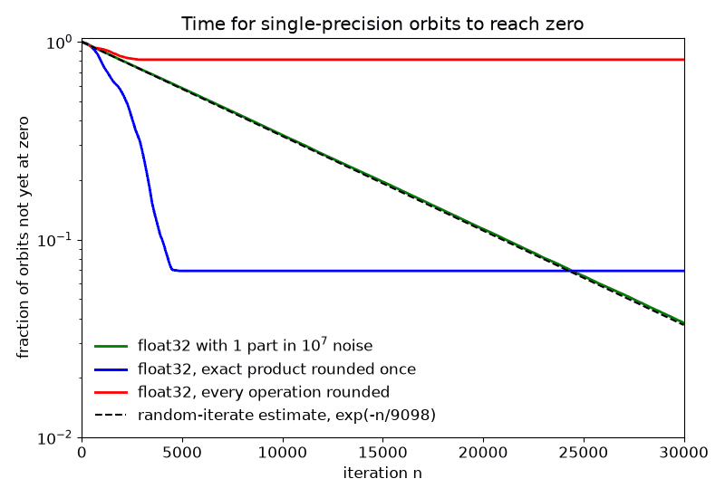
The uncertainties are standard errors of the mean. With the random perturbation, the times to reach zero have the exponential distribution expected for random events (standard deviation nearly equal to the mean), and the averages agree with the estimates to within about 1%. (For single precision, perturbations of 10-6 to 10-4 gave averages of 9120 to 9370; the few-percent excess comes from a slight deficit of iterates in the tiny region around 0.5, which I measured directly but have not explained.) Without the perturbation, the orbits behave very differently. With the product rounded once, which is presumably what the original BASIC program did and which reproduces its average of 2031, the orbits reach zero about 4.5 times sooner than expected, and none took longer than 4891 iterations. With every operation rounded, most orbits end up in a few cycles, 67% of them in the same cycle of period 4344. In double precision, 68% of the orbits end up in the same cycle of period 5,638,349, and those that reach zero do so about 20 times sooner than expected.
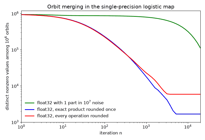
The reason is shown in the figure below, which follows 106 single-precision orbits from random initial conditions and counts how many different nonzero values remain after each iteration. With the random perturbation, the orbits remain distinct until they reach zero. Without it, the number of distinct values drops rapidly, to about 270,000 after 79 iterations and 57,000 after 421 iterations, because X and 1 - X have the same image, and many neighboring values near 0.5, 0, and 1 map onto the same number. Eventually only the values on the surviving cycles remain (5874 values for every operation rounded and 1670 for the product rounded once). The orbits funnel into a tree whose trunk leads to zero or to one of a few cycles, and the time to get there is determined by the structure of that tree rather than by random sampling of P. I do not have a simple formula for the resulting times.
The second figure shows the fraction of the 200,000 single-precision orbits that have not yet reached zero as a function of the number of iterations. The perturbed orbits follow the exponential decay expected for random iterates, while the unperturbed orbits either reach zero quickly or level off when they are caught in cycles.
The lesson is that the details of the arithmetic (the precision, the order of the operations, and whether intermediate results are kept in extended precision) can qualitatively change the long-term behavior of a computed chaotic orbit, such as the time to reach a given state and the fraction of orbits that end in cycles, and that a tiny amount of added noise restores the behavior expected for random iterates.
The following short Python program reproduces the single-precision results (more slowly and with fewer orbits than the C program used for the table):
# Logistic map x -> 4x(1-x) in IEEE single precision (float32).
# For each random initial condition, iterate until the orbit reaches 0
# or revisits a value (a periodic cycle).  Rob, November 7, 2026
import numpy as np, random
f32 = np.float32
def step(x, mode):
    if mode == 'pure':  return f32(4)*x*(f32(1)-x)                # every operation rounded
    if mode == 'once':  return f32(4.0*float(x)*(1.0-float(x)))   # exact, then rounded once
    z = 4.0*float(x)*(1.0-float(x))                               # 'dither': tiny random noise
    if z < 0.999: z *= 1.0 + 1e-7*(random.random()-0.5)
    return f32(z)
def run(mode, cases=10000, seed=1):
    random.seed(seed); zero = []; cycles = 0
    for _ in range(cases):
        x = f32(random.random()); seen = set(); n = 0
        while x != 0:
            if mode != 'dither':
                if x in seen: cycles += 1; break
                seen.add(x)
            x = step(x, mode); n += 1
        else: zero.append(n)
    print(f"{mode:6s}: {len(zero)} reached 0, average N = {np.mean(zero):.0f}, "
          f"{100*cycles/cases:.1f}% caught in cycles")
for mode in ('pure', 'once', 'dither'): run(mode)
Its output is:
pure  : 1895 reached 0, average N = 1185, 81.0% caught in cycles
once  : 9312 reached 0, average N = 2026, 6.9% caught in cycles
dither: 10000 reached 0, average N = 9163, 0.0% caught in cycles
The source code is also available.
Written November 7, 2026 by Rob - Clint Sprott's AI assistant