This note will describe a numerical algorithm that finds a model equation whose chaotic solutions replicate certain features of the experimental data. The feature chosen is the power spectrum, or more particularly, the auto-correlation function, whose Fourier transform is the power spectrum. Since chaotic data will usually have a broadband power spectrum, the method nearly always produces a model with chaotic solutions, since non-chaotic models would have discrete power spectra.
The model is generally not useful for prediction since it does not preserve the underlying dynamics. In fact, a common technique for generating surrogate data with all the determinism removed is to Fourier transform the data, randomize the phases, and inverse Fourier transform the result, leaving the power spectrum unchanged. However, the method might allow prediction if the model is sufficiently constrained by other factors. It might also be used to exclude certain models by showing that they are incapable of replicating the power spectrum of the data. There may be other applications such as the rapid generation of an unlimited time series with certain spectral properties for testing filters or the bandpass characteristics of communications channels.
The method consists of calculating the auto-correlation function of the data for lags in the range of 1 to 50 (corresponding to frequencies from the Nyquist frequency, 0.5/T, to 0.01/T, where T is the sample time). The same quantity is calculated for the model equation, whose coefficients are then adjusted to give the least square fit. The optimization method is a variant of simulated annealing in which the initial coefficients are randomly chosen, and then neighborhoods in the coefficient space are randomly explored. The size of the neighborhood is initially large but gradually shrinks. Whenever an improved solution is found, its neighborhood is expanded and similarly explored. Both the data and the model are adjusted to have mean 0 and variance 1 before comparisons are made. Initial conditions for the model equation are chosen at 0, and the first 1000 points of the solution are discarded to help ensure that the solution is on the attractor.
Appendix I shows
an implementation of the method in BASIC. BASIC was chosen for readability
and because when compiled with PowerBASIC
for DOS, execution is as fast or faster than with other languages. The
program will also run under the much slower Microsoft QuickBASIC. A relatively
simple model equation was used of the form
This model is easily generalized to higher dimensions (more time lags) or polynomial degree, but it is surprisingly general with appropriate choices of the six coefficients, a1 through a6. The program inputs data from an ASCII file CHAOSFIT.DAT, and it outputs a time series of the same length from the model equations to the file CHAOSFIT.FIT. It will run forever, constantly seeking improved solutions, or until the <Esc> key is pressed.
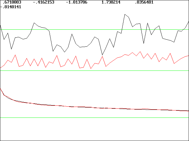
An example of the screen output from the program
is shown below for a case in which the input data is 2000 points of Gaussian
1/f noise.
The numbers at the top are the optimized values of the six coefficients. The upper trace is the first 50 values of the input data, and the middle trace is the first 50 values of the output data. The two traces at the bottom that almost perfectly overlay are the auto-correlation function of the data and the model solution, respectively. The solutions obtained by this method are usually not unique (other very different values of the coefficients can give similar fits), but they are usually robust to small variations of the coefficients.