Fig. 1. Schematic diagram of the circuit described by Eq. (6). The box labeled D(x) represents a nonlinear subcircuit. Nominal values for the unlabeled resistors and capacitors are R = 47 k and C = 1 µF. Approximate values for the input voltage and resistor are V0 = 0.250 V and R0 = 157 k . Also, V1 = and V2 = . The experiment employs dual LMC6062 operational amplifiers, chosen for their high input impedance. Power supplies for the operational amplifiers are tied capacitively to ground to reduce the effects of noise on the circuit.
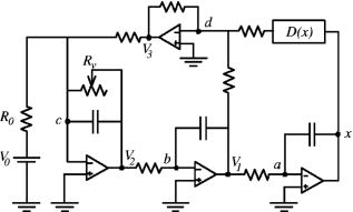
Fig. 2. Schematic diagram of the subcircuit in the box in Fig. 1. The relation between the output and input voltages is given by Vout = D(Vin) = (R2/R1)min(Vin,0).
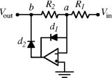
Fig. 3. Experimental measurement of the function D(x) for the nonlinear subcircuit shown in Fig. 2. The superimposed line shows the function defined in Eq. (9). Both x and D(x) are in volts.
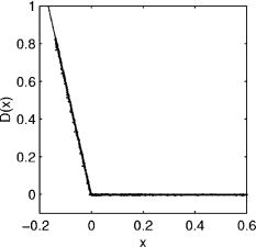
Fig. 4. Experimental, theoretical, and superimposed bifurcation plots for the circuit in Figs. 1 and 2.
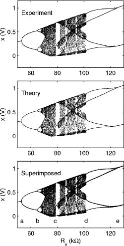
Fig. 5. An expanded view of part of the experimental bifurcation plot shown in Fig. 4.
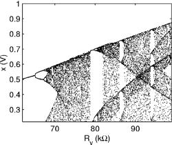
Fig. 6. Experimental power spectral density plots showing the period-doubling route to chaos as Rv is increased. The value of Rv is indicated in the lower left corner. The inset in each plot shows a sample of the experimental time series data used to generate the corresponding spectral density. The smoother line in the period-one plot shows the theoretical spectral density.
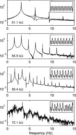
Fig. 7. Experimental phase portraits for several different values of the variable resistance Rv. In each plot x and are plotted (in volts) on the horizontal and vertical axes, respectively. A theoretical curve is superimposed on the period-six case for comparison, although the curve is not distinguishable from the experimental curve. The period-10 attractor comes from a narrow window that is barely discernible at the far right edge of Fig. 5.
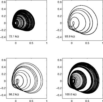
Fig. 8. Stereoscopic plot of the chaotic attractor at Rv = 72.1 k . The x and coordinates are taken from experimental data. The third coordinate is proportional to and is determined numerically by using pairs of values.
Fig. 9. First- and second-return maps for Rv = 72.1 k , taken from experimental data. The insets are magnified by a factor of approximately 6.5 and show the fractal structure of the plots. The intersections of the return maps with the diagonal lines give evidence for (unstable) period-one and -two orbits in the data sets. Such orbits do indeed exist, as seen in Fig. 10.
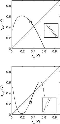
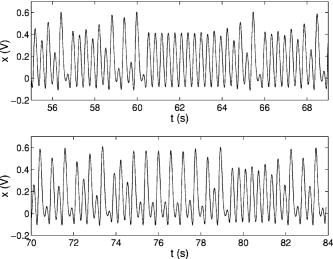
Fig. 10. Experimental wave forms showing unstable period-one and -two orbits within the chaotic time series data for Rv = 72.1 k . The top plot shows an unstable period-one orbit starting shortly after t = 60 s, with a maximum near 0.41 V. The bottom plot shows an unstable period-two orbit starting just before t = 75 s, with maxima near 0.57 V and 0.10 V. The plots themselves are taken from different datasets.