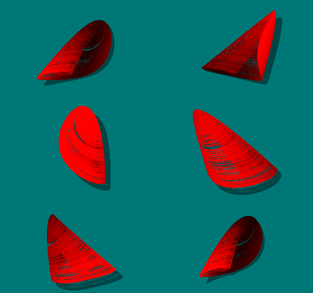
dx/dt = y + z
dy/dt = -x + ay
dz/dt = x2 - bz
Animated view of the
strange attractor for
a = 0.5, b = 1:

In 1994 I proposed 14 simple 3-D chaotic flows with six terms and
one quadratic nonlinearity, called Cases F - S: J. C.
Sprott, Phys. Rev. E 50, R647-R650 (1994).
Through linearly rescaling of the three variables and time,
coefficients of four of the six terms can be made unity, which
means that the systems are completely described by only two
parameters. What follows are plots of the dynamic regions in this
2-D parameter space in which initial conditions are chosen from a
Gaussian distribution of random numbers with mean zero and
variance one, except that the unbounded regions are tested many
times to try to find initial conditions that lead to an attractor.
In the plots, red indicates stable equilibria (S), cyan indicates
periodic limit cycles (P), black indicates chaotic strange
attractors (C), and white indicates unbounded orbits (U). The
original motivation of this study was to identify candidate cases
that exhibit multistability (two coexisting attractors), which
would be indicated by a dotted region in the plane. However, do
not confuse embedded periodic windows in the chaotic regions or
long duration transients with multistability. The best candidate
for coexisting strange attractors and limit cycles appears to be
case P.
| Case F: dx/dt = y + z dy/dt = -x + ay dz/dt = x2 - bz Animated view of the strange attractor for a = 0.5, b = 1:  |
 |
| Case G: dx/dt = ax + bz dy/dt = xz - y dz/dt = -x + y Animated view of the strange attractor for a = 0.4, b = 1:  |
 |
| Case H: dx/dt = -y + z2 dy/dt = x + ay dz/dt = x - bz Animated view of the strange attractor for a = 0.5, b = 1: 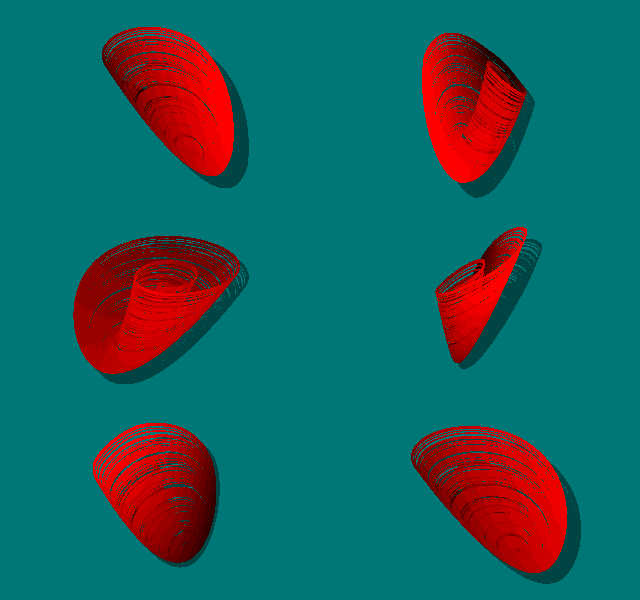 |
 |
| Case I: dx/dt = -ay dy/dt = x + z dz/dt = x + y2 - bz Animated view of the strange attractor for a = 0.2, b = 1:  |
 |
| Case J: dx/dt = az dy/dt = -by + z dz/dt = -x + y + y2 Animated view of the strange attractor for a = 2, b = 2: 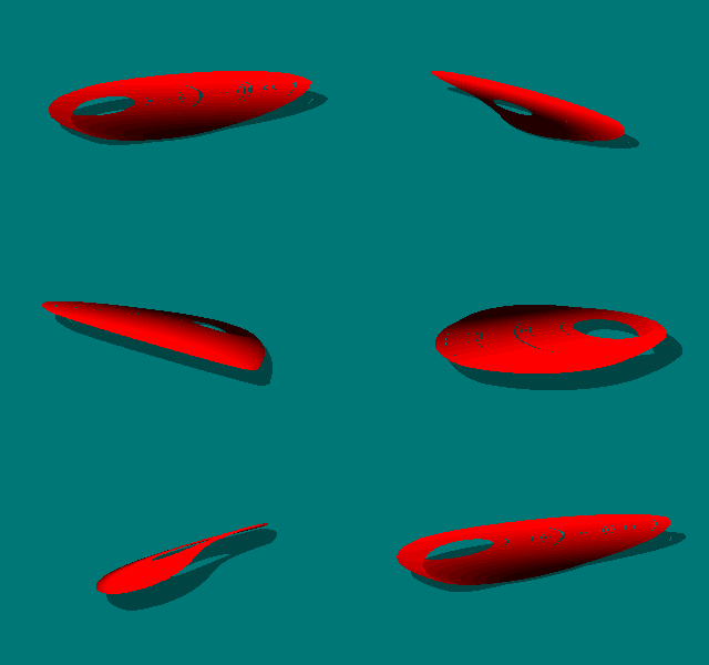 |
 |
| Case K: dx/dt = xy - z dy/dt = x - y dz/dt = ax + bz Animated view of the strange attractor for a = 1, b = 0.3: 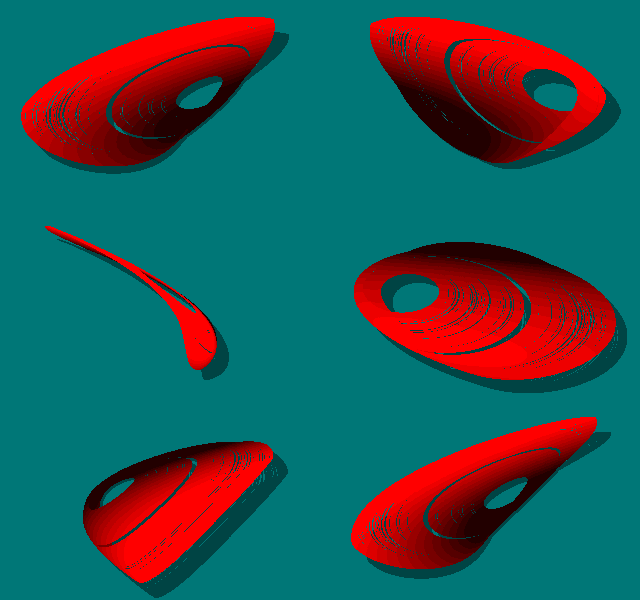 |
 |
| Case L: dx/dt= y + az dy/dt= 0.9x2 - y dz/dt = b - x Animated view of the strange attractor for a = 3.9, b = 1:  |
 |
| Case M: dx/dt = -z dy/dt = -x2 - y dz/dt = a + bx + y Animated view of the strange attractor for a = 1.7, b = 1.7:  |
 |
| Case N: dx/dt = -ay dy/dt = x + z2 dz/dt = 1 + y - bz Animated view of the strange attractor for a = 2, b = 2:  |
 |
| Case O: dx/dt = y dy/dt = x - z dz/dt = ax + xz + by Animated view of the strange attractor for a = 1, b = 2.7:  |
 |
| Case P: dx/dt = ay + z dy/dt = -x + y2 dz/dt = x + by Animated view of the strange attractor for a = 2.7, b = 1:  |
 |
| Case Q: dx/dt = -z dy/dt = x - y dz/dt = ax + y2 + bz Animated view of the strange attractor for a = 3.1, b = 0.5: 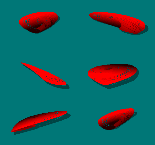 |
 |
| Case R: dx/dt = a - y dy/dt = b + z dz/dt = xy - z Animated view of the strange attractor for a = 0.9, b = 0.4:  |
 |
| Case S: dx/dt = -x - ay dy/dt = x + z2 dz/dt = b + x Animated view of the strange attractor for a = 4, b = 1: 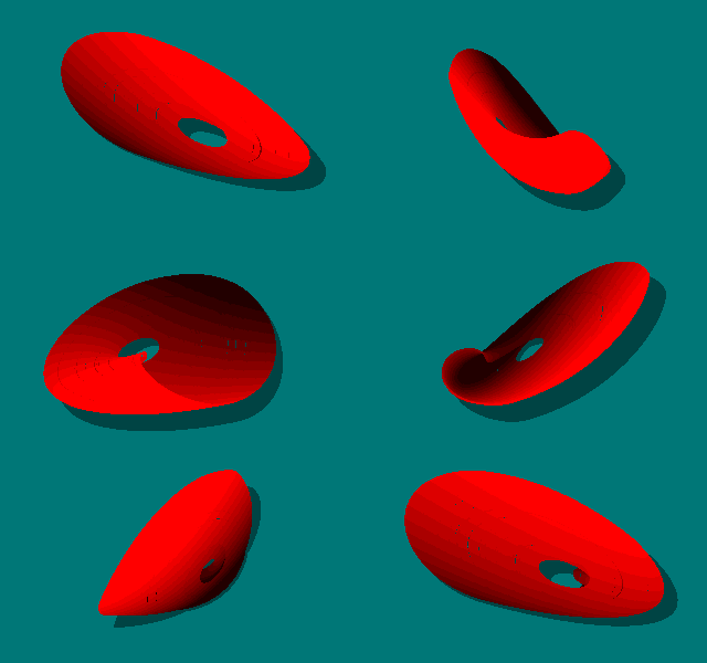 |
 |